Dask DataFrame - 并行化的 pandas
目录
你可以在 live session 中运行此 notebook ![]() ,或在 Github 上查看。
,或在 Github 上查看。

Dask DataFrame - 并行化的 pandas
看起来和用起来都像 pandas API,但适用于并行和分布式工作流。
其核心是,dask.dataframe 模块实现了一个“块并行”的 DataFrame 对象,它看起来和用起来都像 pandas API,但适用于并行和分布式工作流。一个 Dask DataFrame 由许多内存中的 pandas DataFrame 组成,这些 DataFrame 沿索引分开。对一个 Dask DataFrame 的操作会触发对组成它的 pandas DataFrame 进行许多 pandas 操作,这种方式考虑了潜在的并行性和内存限制。

相关文档
何时使用 dask.dataframe
pandas 非常适合内存中可以容纳的表格数据集。使用 pandas 的经验法则是
- “RAM 容量应为数据集大小的 5 到 10 倍”
Wes McKinney (2017) 在 《我讨厌 pandas 的 10 件事》中提到
这里的“数据集大小”是指数据集在磁盘上的大小。
当数据集超出上述规则时,Dask 就变得很有用了。
在本 notebook 中,你将使用纽约市航空公司数据。这个数据集只有大约 200MB,因此你可以在合理的时间内下载它,但是 dask.dataframe 可以扩展到远大于内存的数据集。
设置本地集群
创建本地 Dask 集群并连接到客户端。暂时不用担心这段代码,你将在分布式 notebook 中学习更多。
[2]:
from dask.distributed import Client

client = Client(n_workers=4)
client
[2]:
客户端
Client-a09c1408-168d-11ee-8f9e-6045bd777373
| 连接方法: 集群对象 | 集群类型: distributed.LocalCluster |
| 仪表板: http://127.0.0.1:8787/status |
集群信息
LocalCluster
7b025946
| 仪表板: http://127.0.0.1:8787/status | 工作节点 4 |
| 总线程数 4 | 总内存: 6.77 GiB |
| 状态: 正在运行 | 使用进程: True |
调度器信息
调度器
Scheduler-25b46997-aa0a-463b-b69f-8d3753677e0b
| 通信: tcp://127.0.0.1:37169 | 工作节点 4 |
| 仪表板: http://127.0.0.1:8787/status | 总线程数 4 |
| 启动时间: 刚才 | 总内存: 6.77 GiB |
工作节点
工作节点: 0
| 通信: tcp://127.0.0.1:43205 | 总线程数 1 |
| 仪表板: http://127.0.0.1:40475/status | 内存: 1.69 GiB |
| Nanny: tcp://127.0.0.1:40919 | |
| 本地目录: /tmp/dask-worker-space/worker-hgbikvnh | |
工作节点: 1
| 通信: tcp://127.0.0.1:41081 | 总线程数 1 |
| 仪表板: http://127.0.0.1:34117/status | 内存: 1.69 GiB |
| Nanny: tcp://127.0.0.1:44109 | |
| 本地目录: /tmp/dask-worker-space/worker-xmnubk_n | |
工作节点: 2
| 通信: tcp://127.0.0.1:40213 | 总线程数 1 |
| 仪表板: http://127.0.0.1:42729/status | 内存: 1.69 GiB |
| Nanny: tcp://127.0.0.1:40083 | |
| 本地目录: /tmp/dask-worker-space/worker-x4yncow5 | |
工作节点: 3
| 通信: tcp://127.0.0.1:36801 | 总线程数 1 |
| 仪表板: http://127.0.0.1:33903/status | 内存: 1.69 GiB |
| Nanny: tcp://127.0.0.1:46061 | |
| 本地目录: /tmp/dask-worker-space/worker-6uui7hwh | |
Dask 诊断仪表板
Dask Distributed 提供了一个有用的仪表板,用于可视化集群和计算的状态。
如果你在 JupyterLab 或 Binder 上,可以使用 Dask JupyterLab 扩展(你的环境中应该已经安装了)来打开仪表板图: * 点击左侧边栏中的 Dask 徽标 * 点击放大镜图标,它会自动连接到活动仪表板(如果不起作用,你可以在字段中输入/粘贴仪表板链接 http://127.0.0.1:8787) * 点击“任务流”(Task Stream)、“进度条”(Progress Bar)和“工作节点内存”(Worker Memory),它们将在新选项卡中打开这些图 * 重新组织选项卡以适应你的工作流程!
或者,点击上面客户端详细信息中显示的仪表板链接:http://127.0.0.1:8787/status。它将在新的浏览器选项卡中打开仪表板。
读取和处理数据集
让我们读取美国过去几年的一些航班数据。这些数据专门针对从纽约市区域三个机场起飞的航班。
[3]:
import os
import dask
按照惯例,我们将模块 dask.dataframe 导入为 dd,并将相应的 DataFrame 对象称为 ddf。
注意:“Dask DataFrame”这个术语有点多重含义。根据上下文,它可以指模块或 DataFrame 对象。为了避免混淆,在本 notebook 中: - dask.dataframe(注意全部小写)指 API,- DataFrame(注意驼峰式大小写)指对象。
以下文件名包含 glob 模式 *,因此路径中匹配该模式的所有文件将被读入同一个 DataFrame。
[4]:
import dask.dataframe as dd

ddf = dd.read_csv(
    os.path.join("data", "nycflights", "*.csv"), parse_dates={"Date": [0, 1, 2]}
)
ddf
[4]:
| 日期 | 星期几 | 出发时间 | 计划出发时间 | 到达时间 | 计划到达时间 | 唯一承运人 | 航班号 | 机尾号 | 实际耗时 | 计划耗时 | 飞行时间 | 到达延误 | 出发延误 | 出发地 | 目的地 | 距离 | 滑入时间 | 滑出时间 | 已取消 | 已备降 | |
|---|---|---|---|---|---|---|---|---|---|---|---|---|---|---|---|---|---|---|---|---|---|
| npartitions=10 | |||||||||||||||||||||
| datetime64[ns] | int64 | float64 | int64 | float64 | int64 | object | int64 | float64 | float64 | int64 | float64 | float64 | float64 | object | object | float64 | float64 | float64 | int64 | int64 | |
| ... | ... | ... | ... | ... | ... | ... | ... | ... | ... | ... | ... | ... | ... | ... | ... | ... | ... | ... | ... | ... | |
| ... | ... | ... | ... | ... | ... | ... | ... | ... | ... | ... | ... | ... | ... | ... | ... | ... | ... | ... | ... | ... | ... |
| ... | ... | ... | ... | ... | ... | ... | ... | ... | ... | ... | ... | ... | ... | ... | ... | ... | ... | ... | ... | ... | |
| ... | ... | ... | ... | ... | ... | ... | ... | ... | ... | ... | ... | ... | ... | ... | ... | ... | ... | ... | ... | ... |
Dask 尚未加载数据,它已完成: - 调查输入路径并发现有十个匹配文件 - 智能地为每个数据块创建了一组作业 - 在本例中,每个原始 CSV 文件对应一个作业
请注意,DataFrame 对象的表示中不包含任何数据 - Dask 仅完成了足以读取第一个文件开头并推断列名和数据类型的工作。
惰性评估
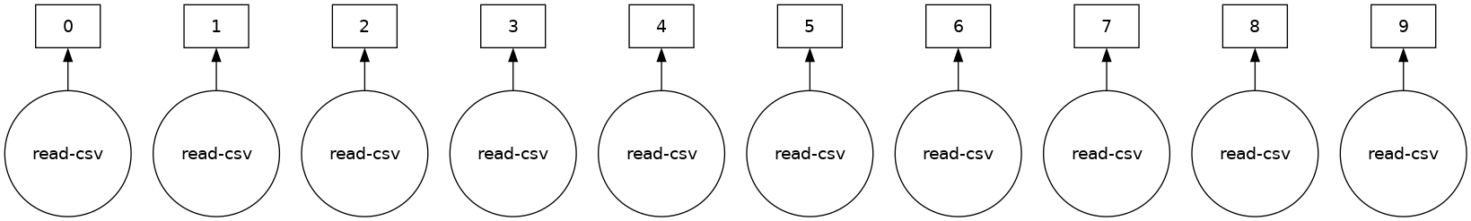
大多数 Dask 集合,包括 Dask DataFrame,都是惰性评估的,这意味着 Dask 会立即构建你的计算逻辑(称为任务图),但只在必要时才“评估”它们。你可以使用 .visualize() 查看此任务图。
你将在 Delayed notebook 中了解更多相关信息,但现在请注意,我们需要调用 .compute() 来触发实际计算。
[5]:
ddf.visualize()
[5]:
一些函数,如 len 和 head,也会触发计算。具体来说,调用 len 会: - 加载实际数据(即,将每个文件加载到 pandas DataFrame 中) - 然后将相应的函数应用于每个 pandas DataFrame(也称为分区) - 合并小计以给出最终总计
[6]:
# load and count number of rows
len(ddf)
[6]:
9990
你可以像在 pandas 中一样查看数据的开头和结尾
[7]:
ddf.head()
[7]:
| 日期 | 星期几 | 出发时间 | 计划出发时间 | 到达时间 | 计划到达时间 | 唯一承运人 | 航班号 | 机尾号 | 实际耗时 | ... | 飞行时间 | 到达延误 | 出发延误 | 出发地 | 目的地 | 距离 | 滑入时间 | 滑出时间 | 已取消 | 已备降 | |
|---|---|---|---|---|---|---|---|---|---|---|---|---|---|---|---|---|---|---|---|---|---|
| 0 | 1990-01-01 | 1 | 1621.0 | 1540 | 1747.0 | 1701 | US | 33 | NaN | 86.0 | ... | NaN | 46.0 | 41.0 | EWR | PIT | 319.0 | NaN | NaN | 0 | 0 |
| 1 | 1990-01-02 | 2 | 1547.0 | 1540 | 1700.0 | 1701 | US | 33 | NaN | 73.0 | ... | NaN | -1.0 | 7.0 | EWR | PIT | 319.0 | NaN | NaN | 0 | 0 |
| 2 | 1990-01-03 | 3 | 1546.0 | 1540 | 1710.0 | 1701 | US | 33 | NaN | 84.0 | ... | NaN | 9.0 | 6.0 | EWR | PIT | 319.0 | NaN | NaN | 0 | 0 |
| 3 | 1990-01-04 | 4 | 1542.0 | 1540 | 1710.0 | 1701 | US | 33 | NaN | 88.0 | ... | NaN | 9.0 | 2.0 | EWR | PIT | 319.0 | NaN | NaN | 0 | 0 |
| 4 | 1990-01-05 | 5 | 1549.0 | 1540 | 1706.0 | 1701 | US | 33 | NaN | 77.0 | ... | NaN | 5.0 | 9.0 | EWR | PIT | 319.0 | NaN | NaN | 0 | 0 |
5 行 × 21 列
ddf.tail()

# ValueError: Mismatched dtypes found in `pd.read_csv`/`pd.read_table`.

# +----------------+---------+----------+
# | Column         | Found   | Expected |
# +----------------+---------+----------+
# | CRSElapsedTime | float64 | int64    |
# | TailNum        | object  | float64  |
# +----------------+---------+----------+

# The following columns also raised exceptions on conversion:

# - TailNum
#   ValueError("could not convert string to float: 'N54711'")

# Usually this is due to dask's dtype inference failing, and
# *may* be fixed by specifying dtypes manually by adding:

# dtype={'CRSElapsedTime': 'float64',
#        'TailNum': 'object'}

# to the call to `read_csv`/`read_table`.
与 pandas.read_csv 在推断数据类型之前读取整个文件不同,dask.dataframe.read_csv 只读取文件开头(或使用 glob 时的第一个文件)的样本。然后在读取所有分区时强制执行这些推断的数据类型。
在这种情况下,样本中推断的数据类型不正确。前 n 行没有 CRSElapsedTime 的值(pandas 将其推断为 float),后来发现是字符串(object dtype)。请注意,Dask 会提供有关不匹配的详细错误消息。发生这种情况时,你有几个选项
使用
dtype关键字直接指定数据类型。这是推荐的解决方案,因为它的错误率最低(显式优于隐式),而且性能最好。增加
sample关键字的大小(以字节为单位)使用
assume_missing让dask假定推断为int(不允许缺失值)的列实际上是float(允许缺失值)。在我们的特定情况下,这不适用。
在我们的例子中,我们将使用第一个选项并直接指定有问题的列的数据类型。
[8]:
ddf = dd.read_csv(
    os.path.join("data", "nycflights", "*.csv"),
    parse_dates={"Date": [0, 1, 2]},
    dtype={"TailNum": str, "CRSElapsedTime": float, "Cancelled": bool},
)
[9]:
ddf.tail() # now works
[9]:
| 日期 | 星期几 | 出发时间 | 计划出发时间 | 到达时间 | 计划到达时间 | 唯一承运人 | 航班号 | 机尾号 | 实际耗时 | ... | 飞行时间 | 到达延误 | 出发延误 | 出发地 | 目的地 | 距离 | 滑入时间 | 滑出时间 | 已取消 | 已备降 | |
|---|---|---|---|---|---|---|---|---|---|---|---|---|---|---|---|---|---|---|---|---|---|
| 994 | 1999-01-25 | 1 | 632.0 | 635 | 803.0 | 817 | CO | 437 | N27213 | 91.0 | ... | 68.0 | -14.0 | -3.0 | EWR | RDU | 416.0 | 4.0 | 19.0 | False | 0 |
| 995 | 1999-01-26 | 2 | 632.0 | 635 | 751.0 | 817 | CO | 437 | N16217 | 79.0 | ... | 62.0 | -26.0 | -3.0 | EWR | RDU | 416.0 | 3.0 | 14.0 | False | 0 |
| 996 | 1999-01-27 | 3 | 631.0 | 635 | 756.0 | 817 | CO | 437 | N12216 | 85.0 | ... | 66.0 | -21.0 | -4.0 | EWR | RDU | 416.0 | 4.0 | 15.0 | False | 0 |
| 997 | 1999-01-28 | 4 | 629.0 | 635 | 803.0 | 817 | CO | 437 | N26210 | 94.0 | ... | 69.0 | -14.0 | -6.0 | EWR | RDU | 416.0 | 5.0 | 20.0 | False | 0 |
| 998 | 1999-01-29 | 5 | 632.0 | 635 | 802.0 | 817 | CO | 437 | N12225 | 90.0 | ... | 67.0 | -15.0 | -3.0 | EWR | RDU | 416.0 | 5.0 | 18.0 | False | 0 |
5 行 × 21 列
从远程存储读取
如果你正在考虑分布式计算,你的数据可能存储在远程服务(如 Amazon S3 或 Google Cloud Storage)上,并且采用更友好的格式(如 Parquet)。Dask 可以直接从这些远程位置以惰性方式并行读取各种格式的数据。
以下是如何从 Amazon S3 读取纽约市出租车数据的方法
ddf = dd.read_parquet(
    "s3://nyc-tlc/trip data/yellow_tripdata_2012-*.parquet",
)
你还可以利用 Parquet 特有的优化,如列选择和元数据处理,在 Dask 关于处理 Parquet 文件的文档中了解更多信息。
使用 dask.dataframe 进行计算
让我们计算航班延误的最大值。
如果只使用 pandas,我们将遍历每个文件以找到各个最大值,然后找到所有各个最大值的最终最大值。
import pandas as pd

files = os.listdir(os.path.join('data', 'nycflights'))

maxes = []

for file in files:
    df = pd.read_csv(os.path.join('data', 'nycflights', file))
    maxes.append(df.DepDelay.max())

final_max = max(maxes)
dask.dataframe 允许我们编写类似 pandas 的代码,对大于内存的数据集进行并行操作。
[10]:
%%time
result = ddf.DepDelay.max()
result.compute()
CPU times: user 25.2 ms, sys: 29 µs, total: 25.2 ms
Wall time: 84.8 ms
[10]:
409.0
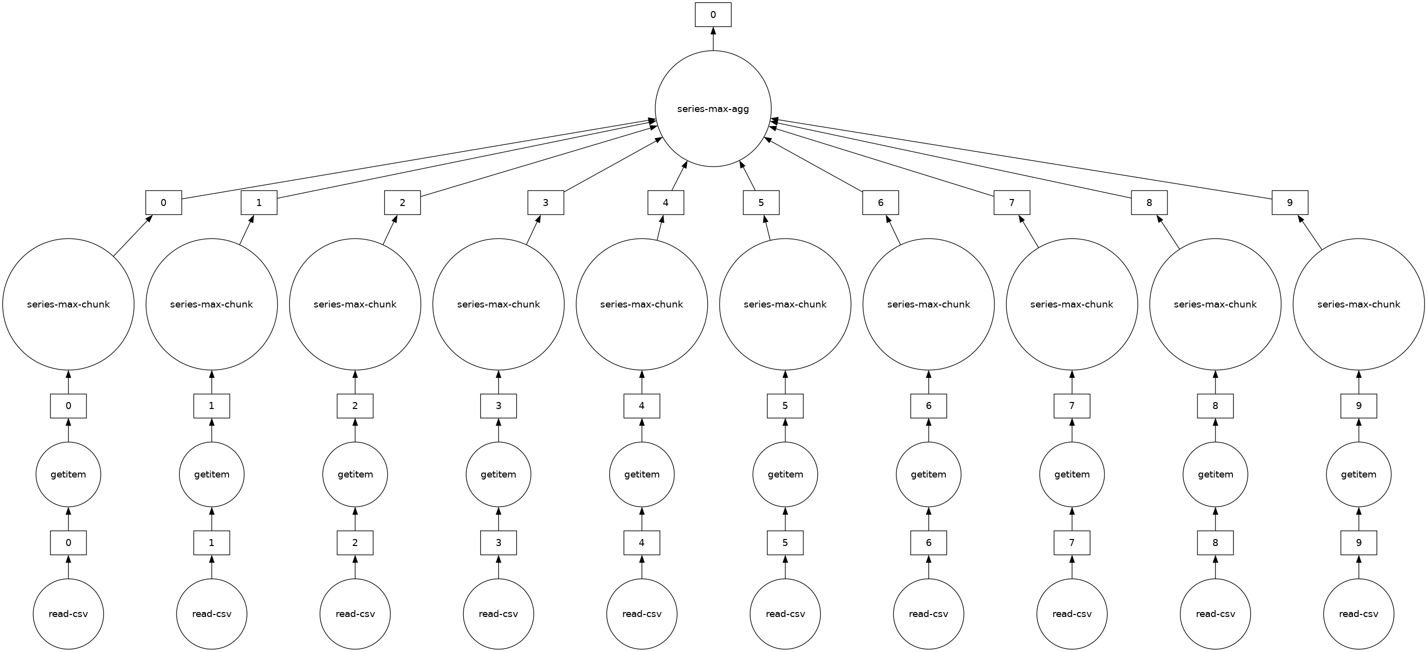
这为我们创建了惰性计算,然后运行它。
注意: Dask 会尽快删除中间结果(例如每个文件的完整 pandas DataFrame)。这意味着你可以处理大于内存的数据集,但是重复计算每次都必须重新加载所有数据。(再次运行上面的代码,它比你预期的快还是慢?)
你可以使用 .visualize() 查看底层任务图
[11]:
# notice the parallelism
result.visualize()
[11]:
练习
在本节中,你将进行一些 dask.dataframe 计算。如果你熟悉 pandas,那么这些应该会很熟悉。你需要考虑何时调用 .compute()。
3. 总共有多少非取消航班从每个机场起飞?
提示:使用groupby。
[16]:
# Your code here
[17]:
ddf[~ddf.Cancelled].groupby("Origin").Origin.count().compute()
[17]:
Origin
EWR    4132
JFK    1085
LGA    4166
Name: Origin, dtype: int64
4. 每个机场的平均出发延误是多少?
[18]:
# Your code here
[19]:
ddf.groupby("Origin").DepDelay.mean().compute()
[19]:
Origin
EWR    12.500968
JFK    17.053456
LGA    10.169227
Name: DepDelay, dtype: float64
5. 一周中哪一天的平均出发延误最严重?
[20]:
# Your code here
[21]:
ddf.groupby("DayOfWeek").DepDelay.mean().idxmax().compute()
[21]:
5
6. 假设距离列有错误,你需要给所有值加 1,你会怎么做?
[22]:
# Your code here
[23]:
ddf["Distance"].apply(
    lambda x: x + 1
).compute()  # don't worry about the warning, we'll discuss in the next sections

# OR

(ddf["Distance"] + 1).compute()
/usr/share/miniconda3/envs/dask-tutorial/lib/python3.10/site-packages/dask/dataframe/core.py:4139: UserWarning:
You did not provide metadata, so Dask is running your function on a small dataset to guess output types. It is possible that Dask will guess incorrectly.
To provide an explicit output types or to silence this message, please provide the `meta=` keyword, as described in the map or apply function that you are using.
  Before: .apply(func)
  After:  .apply(func, meta=('Distance', 'float64'))

  warnings.warn(meta_warning(meta))
[23]:
0      320.0
1      320.0
2      320.0
3      320.0
4      320.0
       ...
994    417.0
995    417.0
996    417.0
997    417.0
998    417.0
Name: Distance, Length: 9990, dtype: float64
共享中间结果
在计算上述所有内容时,我们有时会多次执行相同的操作。对于大多数操作,dask.dataframe 会存储参数,从而允许共享重复的计算并仅计算一次。
例如,让我们计算所有非取消航班的出发延误的平均值和标准差。由于 Dask 操作是惰性的,这些值还不是最终结果。它们只是获取结果所需的步骤。
如果你通过两次调用 compute 来计算它们,则不会共享中间计算。
[24]:
non_canceled = ddf[~ddf.Cancelled]
mean_delay = non_canceled.DepDelay.mean()
std_delay = non_canceled.DepDelay.std()
[25]:
%%time

mean_delay_res = mean_delay.compute()
std_delay_res = std_delay.compute()
CPU times: user 78.7 ms, sys: 4.18 ms, total: 82.9 ms
Wall time: 237 ms
dask.compute
但让我们尝试将两者都传递给一次 compute 调用。
[26]:
%%time

mean_delay_res, std_delay_res = dask.compute(mean_delay, std_delay)
CPU times: user 54.1 ms, sys: 0 ns, total: 54.1 ms
Wall time: 147 ms
使用 dask.compute 大约只需要一半的时间。这是因为在调用 dask.compute 时,两个结果的任务图会合并,从而允许共享操作只执行一次而不是两次。特别是,使用 dask.compute 只会执行以下操作一次
对
read_csv的调用过滤 (
df[~df.Cancelled])一些必要的归约 (
sum,count)
要查看多个结果之间的合并任务图是什么样的(以及哪些被共享了),你可以使用 dask.visualize 函数(你可能想使用 filename='graph.pdf' 将图保存到磁盘以便更容易放大查看)
[27]:
dask.visualize(mean_delay, std_delay, engine="cytoscape")
[27]:
.persist()
在使用分布式调度器时(你将在后续 notebook 中了解更多关于调度器的信息),你可以将一些你想经常使用的数据保存在分布式内存中。
persist 生成“Futures”(稍后也会详细介绍)并将它们存储在与你的输出相同的结构中。你可以对任何适合内存的数据或计算使用 persist。
如果你只想分析从 JFK 机场起飞的非取消航班的数据,你可以像上一节一样进行两次 compute 调用
[28]:
non_cancelled = ddf[~ddf.Cancelled]
ddf_jfk = non_cancelled[non_cancelled.Origin == "JFK"]
[29]:
%%time
ddf_jfk.DepDelay.mean().compute()
ddf_jfk.DepDelay.sum().compute()
CPU times: user 74.6 ms, sys: 0 ns, total: 74.6 ms
Wall time: 244 ms
[29]:
18503.0
或者,考虑将该数据子集持久化到内存中。
查看“图”(Graph)仪表板图,红色方块表示作为 Futures 存储在内存中的持久化数据。你还会注意到工作节点内存(Worker Memory,另一个仪表板图)消耗的增加。
[30]:
ddf_jfk = ddf_jfk.persist() # returns back control immediately
[31]:
%%time
ddf_jfk.DepDelay.mean().compute()
ddf_jfk.DepDelay.std().compute()
CPU times: user 83.8 ms, sys: 4.65 ms, total: 88.4 ms
Wall time: 208 ms
[31]:
36.85799641792652
对这些持久化数据的分析更快,因为我们不必重复加载和选择(非取消、从 JFK 出发)操作。
使用 Dask DataFrame 的自定义代码
dask.dataframe 只涵盖了 pandas API 中一小部分但常用功能。
此限制有两个原因
Pandas API 非常庞大
有些操作确实难以并行化,例如排序。
此外,一些重要的操作,如 set_index,虽然可以工作,但比在 pandas 中慢,因为它们涉及到大量的数据混洗,并可能写入磁盘。
如果你想使用一些尚未(或无法)为 Dask DataFrame 实现的自定义函数怎么办?
你可以在 Dask 问题跟踪器上提交问题,检查该函数实现的可能性,并可以考虑为 Dask 贡献该函数。
如果它是自定义函数或实现起来很复杂,dask.dataframe 提供了一些方法来使将自定义函数应用于 Dask DataFrames 更容易
`map_partitions<https://docs.dask.org.cn/en/latest/generated/dask.dataframe.DataFrame.map_partitions.html>`__: 在 Dask DataFrame 的每个分区(即每个 pandas DataFrame)上运行函数`map_overlap<https://docs.dask.org.cn/en/latest/generated/dask.dataframe.rolling.map_overlap.html>`__: 在 Dask DataFrame 的每个分区(即每个 pandas DataFrame)上运行函数,相邻分区之间共享一些行`reduction<https://docs.dask.org.cn/en/latest/generated/dask.dataframe.Series.reduction.html>`__: 用于自定义的按行归约操作。
让我们快速了解一下 map_partitions() 函数
[32]:
help(ddf.map_partitions)
Help on method map_partitions in module dask.dataframe.core:

map_partitions(func, *args, **kwargs) method of dask.dataframe.core.DataFrame instance
    Apply Python function on each DataFrame partition.

    Note that the index and divisions are assumed to remain unchanged.

    Parameters
    ----------
    func : function
        The function applied to each partition. If this function accepts
        the special ``partition_info`` keyword argument, it will receive
        information on the partition's relative location within the
        dataframe.
    args, kwargs :
        Positional and keyword arguments to pass to the function.
        Positional arguments are computed on a per-partition basis, while
        keyword arguments are shared across all partitions. The partition
        itself will be the first positional argument, with all other
        arguments passed *after*. Arguments can be ``Scalar``, ``Delayed``,
        or regular Python objects. DataFrame-like args (both dask and
        pandas) will be repartitioned to align (if necessary) before
        applying the function; see ``align_dataframes`` to control this
        behavior.
    enforce_metadata : bool, default True
        Whether to enforce at runtime that the structure of the DataFrame
        produced by ``func`` actually matches the structure of ``meta``.
        This will rename and reorder columns for each partition,
        and will raise an error if this doesn't work,
        but it won't raise if dtypes don't match.
    transform_divisions : bool, default True
        Whether to apply the function onto the divisions and apply those
        transformed divisions to the output.
    align_dataframes : bool, default True
        Whether to repartition DataFrame- or Series-like args
        (both dask and pandas) so their divisions align before applying
        the function. This requires all inputs to have known divisions.
        Single-partition inputs will be split into multiple partitions.

        If False, all inputs must have either the same number of partitions
        or a single partition. Single-partition inputs will be broadcast to
        every partition of multi-partition inputs.
    meta : pd.DataFrame, pd.Series, dict, iterable, tuple, optional
        An empty ``pd.DataFrame`` or ``pd.Series`` that matches the dtypes
        and column names of the output. This metadata is necessary for
        many algorithms in dask dataframe to work.  For ease of use, some
        alternative inputs are also available. Instead of a ``DataFrame``,
        a ``dict`` of ``{name: dtype}`` or iterable of ``(name, dtype)``
        can be provided (note that the order of the names should match the
        order of the columns). Instead of a series, a tuple of ``(name,
        dtype)`` can be used. If not provided, dask will try to infer the
        metadata. This may lead to unexpected results, so providing
        ``meta`` is recommended. For more information, see
        ``dask.dataframe.utils.make_meta``.

    Examples
    --------
    Given a DataFrame, Series, or Index, such as:

    >>> import pandas as pd
    >>> import dask.dataframe as dd
    >>> df = pd.DataFrame({'x': [1, 2, 3, 4, 5],
    ...                    'y': [1., 2., 3., 4., 5.]})
    >>> ddf = dd.from_pandas(df, npartitions=2)

    One can use ``map_partitions`` to apply a function on each partition.
    Extra arguments and keywords can optionally be provided, and will be
    passed to the function after the partition.

    Here we apply a function with arguments and keywords to a DataFrame,
    resulting in a Series:

    >>> def myadd(df, a, b=1):
    ...     return df.x + df.y + a + b
    >>> res = ddf.map_partitions(myadd, 1, b=2)
    >>> res.dtype
    dtype('float64')

    Here we apply a function to a Series resulting in a Series:

    >>> res = ddf.x.map_partitions(lambda x: len(x)) # ddf.x is a Dask Series Structure
    >>> res.dtype
    dtype('int64')

    By default, dask tries to infer the output metadata by running your
    provided function on some fake data. This works well in many cases, but
    can sometimes be expensive, or even fail. To avoid this, you can
    manually specify the output metadata with the ``meta`` keyword. This
    can be specified in many forms, for more information see
    ``dask.dataframe.utils.make_meta``.

    Here we specify the output is a Series with no name, and dtype
    ``float64``:

    >>> res = ddf.map_partitions(myadd, 1, b=2, meta=(None, 'f8'))

    Here we map a function that takes in a DataFrame, and returns a
    DataFrame with a new column:

    >>> res = ddf.map_partitions(lambda df: df.assign(z=df.x * df.y))
    >>> res.dtypes
    x      int64
    y    float64
    z    float64
    dtype: object

    As before, the output metadata can also be specified manually. This
    time we pass in a ``dict``, as the output is a DataFrame:

    >>> res = ddf.map_partitions(lambda df: df.assign(z=df.x * df.y),
    ...                          meta={'x': 'i8', 'y': 'f8', 'z': 'f8'})

    In the case where the metadata doesn't change, you can also pass in
    the object itself directly:

    >>> res = ddf.map_partitions(lambda df: df.head(), meta=ddf)

    Also note that the index and divisions are assumed to remain unchanged.
    If the function you're mapping changes the index/divisions, you'll need
    to clear them afterwards:

    >>> ddf.map_partitions(func).clear_divisions()  # doctest: +SKIP

    Your map function gets information about where it is in the dataframe by
    accepting a special ``partition_info`` keyword argument.

    >>> def func(partition, partition_info=None):
    ...     pass

    This will receive the following information:

    >>> partition_info  # doctest: +SKIP
    {'number': 1, 'division': 3}

    For each argument and keyword arguments that are dask dataframes you will
    receive the number (n) which represents the nth partition of the dataframe
    and the division (the first index value in the partition). If divisions
    are not known (for instance if the index is not sorted) then you will get
    None as the division.
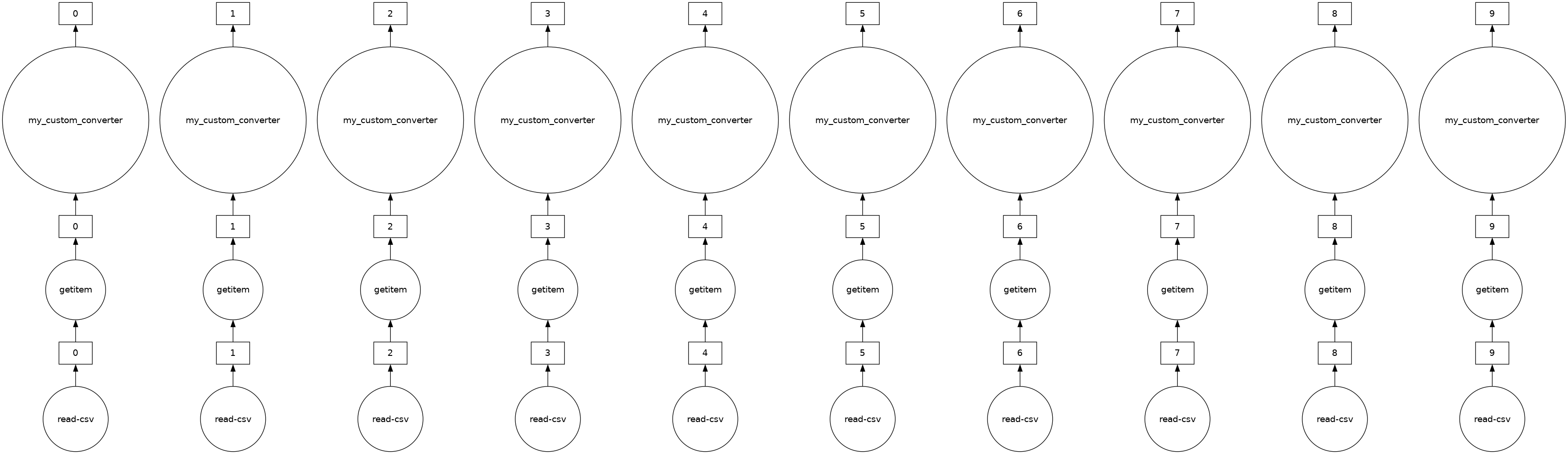
ddf 中的“距离”列当前以英里为单位。假设我们想将单位转换为公里,并且我们有一个通用的辅助函数,如下所示。在这种情况下,我们可以使用 map_partitions 并行地将此函数应用于每个内部 pandas DataFrame。
[33]:
def my_custom_converter(df, multiplier=1):
    return df * multiplier


meta = pd.Series(name="Distance", dtype="float64")

distance_km = ddf.Distance.map_partitions(
    my_custom_converter, multiplier=0.6, meta=meta
)
[34]:
distance_km.visualize()
[34]:
[35]:
distance_km.head()
[35]:
0    191.4
1    191.4
2    191.4
3    191.4
4    191.4
Name: Distance, dtype: float64
什么是 meta?
由于 Dask 是惰性操作的,它并不总是有足够的信息来推断某些操作的输出结构(包括数据类型)。
meta 是关于你的计算输出对 Dask 的一个建议。重要的是,meta 永远不会干预输出结构。Dask 会使用这个 meta,直到它能够确定实际的输出结构。
尽管有很多方法来定义 meta,我们建议使用一个与最终输出结构匹配的小型 pandas Series 或 DataFrame。